⚛️ Schrödinger Wave Equation: Derivation from Classical Wave Theory
The Schrödinger equation is the fundamental pillar of quantum mechanics. It describes how the quantum state of a physical system changes with time. Unlike classical physics, which uses deterministic trajectories, the Schrödinger equation yields a wavefunction \(\psi\) whose square modulus gives the probability density of finding a particle at a given location. It naturally explains quantized energy levels, wave‑particle duality, and the structure of atoms and molecules.
🌊 DIAGRAM 1: Wave‑particle duality – an electron behaves both as a particle and a matter wave.
[Illustration: a particle-like dot and a sinusoidal wave superimposed, symbolizing the dual nature]
📜 What the Schrödinger Equation Represents
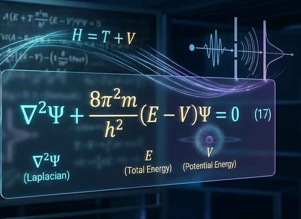
At its core, the equation treats particles (e.g., electrons) as wavefunctions \(\Psi(\mathbf{r}, t)\). Instead of a hard point moving through space, the electron is viewed as a “probability cloud”. The equation allows us to calculate how this wave evolves under the influence of forces (potential energy). The time‑independent form for a single particle of mass \(m\) in a potential \(V(\mathbf{r})\) is:
where \(\nabla^2 = \frac{\partial^2}{\partial x^2} + \frac{\partial^2}{\partial y^2} + \frac{\partial^2}{\partial z^2}\) is the Laplacian operator, \(E\) is the total energy, and \(h\) is Planck’s constant.
🔬 Why It’s Revolutionary
- Foundation of Chemistry: Every chemical bond and periodic trend emerges from solutions to this equation.
- Quantization: Explains why electrons in atoms exist only at discrete energy levels.
- Wave‑Particle Duality: Unifies the classical concepts of particle and wave mathematically.
📐 Step‑by‑Step Derivation from Classical Wave Equation
The Schrödinger equation can be derived by merging the classical wave equation with de Broglie’s hypothesis of matter waves. Below is a detailed, step‑wise derivation for the time‑independent form.
For a wave traveling along the \(x\)-axis with phase velocity \(v\), the displacement \(y(x,t)\) obeys: \[ \frac{\partial^2 y}{\partial x^2} = \frac{1}{v^2} \frac{\partial^2 y}{\partial t^2} \quad \text{(1)} \]
For a stationary (standing) wave, we separate spatial and temporal parts: \[ y(x,t) = f(x) \, f'(t) \] For harmonic motion, \(f'(t) = A \sin(2\pi \nu t)\), where \(\nu\) is frequency.
\[ \frac{\partial^2 y}{\partial t^2} = -4\pi^2 \nu^2 f(x) f'(t) \quad \text{(2)} \]
\[ \frac{\partial^2 y}{\partial x^2} = f'(t) \frac{d^2 f}{dx^2} \quad \text{(3)} \]
\[ f'(t) \frac{d^2 f}{dx^2} = \frac{1}{v^2} \left[ -4\pi^2 \nu^2 f(x) f'(t) \right] \] Cancel \(f'(t)\) (non‑zero) and use \(v = \nu \lambda\): \[ \frac{d^2 f}{dx^2} = -\frac{4\pi^2 \nu^2}{v^2} f(x) = -\frac{4\pi^2}{\lambda^2} f(x) \] Replacing \(f(x)\) with the wavefunction \(\psi(x)\): \[ \frac{d^2 \psi}{dx^2} = -\frac{4\pi^2}{\lambda^2} \psi \quad \text{(4)} \]
de Broglie proposed that any particle of momentum \(p = mv\) has a wavelength \(\lambda = \frac{h}{mv}\). Hence \(\frac{1}{\lambda^2} = \frac{m^2 v^2}{h^2}\). Substitute into (4): \[ \frac{d^2 \psi}{dx^2} = -\frac{4\pi^2 m^2 v^2}{h^2} \psi \] Rearranged: \[ \frac{d^2 \psi}{dx^2} + \frac{4\pi^2 m^2 v^2}{h^2} \psi = 0 \quad \text{(5)} \]
Total energy \(E = \frac{1}{2}mv^2 + V\). Thus \(mv^2 = 2(E – V)\), and \(m^2 v^2 = 2m(E – V)\). Substitute into (5): \[ \frac{d^2 \psi}{dx^2} + \frac{4\pi^2 \cdot 2m(E – V)}{h^2} \psi = 0 \] \[ \frac{d^2 \psi}{dx^2} + \frac{8\pi^2 m}{h^2}(E – V)\psi = 0 \quad \text{(6)} \]
In three dimensions, the second derivative becomes the Laplacian: \[ \nabla^2 \psi + \frac{8\pi^2 m}{h^2}(E – V)\psi = 0 \] which is the time‑independent Schrödinger equation.
🎸 DIAGRAM 2: Standing waves on a string – fundamental mode and overtones. These illustrate quantized wavelengths, analogous to electron orbitals.
[Schematic: fixed ends showing nodes (points of zero displacement) and antinodes]
💡 Physical Interpretation of the Wavefunction
The wavefunction \(\psi(\mathbf{r})\) itself is not directly observable. However, the quantity \(|\psi(\mathbf{r})|^2 dV\) gives the probability of finding the particle in a small volume \(dV\) around \(\mathbf{r}\). This interpretation, due to Max Born, is a cornerstone of quantum mechanics. The wavefunction must be single‑valued, continuous, and normalizable (total probability = 1).
📊 DIAGRAM 3: Probability cloud of an electron in the 1s orbital of hydrogen (radial distribution).
[Density plot showing higher density near the nucleus, fading outward]
✅ Applications and Successes
- Hydrogen atom: Exact solution gives quantized energy levels \(E_n = -13.6/n^2\) eV, matching Bohr model and experiment.
- Quantum tunneling: Explains alpha decay, scanning tunneling microscopy (STM).
- Chemical bonding: Solutions for molecules (molecular orbitals) explain bond formation.
- Solid‑state physics: Band theory of solids arises from Schrödinger equation in periodic potentials.
⚠️ Limitations and Advanced Extensions
- The non‑relativistic form fails at very high energies (speeds close to light). Dirac equation (1928) incorporates relativity and spin.
- For many‑electron systems, the equation becomes analytically unsolvable; approximations (Hartree‑Fock, density functional theory) are used.
- Interpretational issues (wavefunction collapse, measurement problem) remain topics of debate.
📘 English lecture slot – will be updated soon. For now, enjoy the detailed Urdu/Hindi explanation.
📚 References & Further Reading
- Griffiths, D. J. (2018). Introduction to Quantum Mechanics. Cambridge University Press.
- Eisberg, R., & Resnick, R. (1985). Quantum Physics of Atoms, Molecules, Solids, Nuclei, and Particles. Wiley.
- Schrödinger, E. (1926). “Quantisierung als Eigenwertproblem” (Quantization as an eigenvalue problem). Annalen der Physik.
- de Broglie, L. (1925). Recherches sur la théorie des quanta (PhD thesis).
Download Complete Notes Below
Proudly Powered By

Leave a Comment