Liquid Junction Potential Explained: Definition, Calculation, Examples, and Applications
In electrochemical systems, the regions where different components meet are often the most critical zones for potential development. One of the most common, yet frequently misunderstood, phenomena occurring at these boundaries is the Liquid Junction Potential (LJP). When two distinct electrolyte solutions or solutions containing different concentrations of the same electrolyte are brought into physical contact, they do not remain static. Instead, an interfacial region forms where ions spontaneously migrate across the boundary. Because distinct ionic species move at unequal velocities due to variations in size, hydration energy, and charge density, a local charge separation is established.
What is Liquid Junction Potential?
Liquid Junction Potential (also referred to as diffusion potential) is defined as the potential difference that develops across the interface of two electrolytic solutions of different compositions or concentrations that are in direct contact. This interface creates a state of thermodynamic non-equilibrium. Because a chemical potential gradient exists across the junction, a spontaneous flux of matter occurs. Ions move from regions of high chemical activity to regions of low chemical activity. This migration process continues until an electrostatic counter-force balances the purely diffusional drive, bringing the system into a steady state.
The Core Mechanism of Generation
To conceptualize how this potential arises, consider a simple system where a concentrated solution of hydrochloric acid (HCl) is placed in direct contact with a highly dilute solution of HCl. The hydrogen ions (H⁺) and chloride ions (Cl⁻) in the concentrated zone instantly begin diffusing toward the dilute zone. The rate at which an ion diffuses is directly proportional to its ionic mobility (u) within an electrical field. The H⁺ ion is exceptionally small and possesses a unique transport mechanism in water, making it much faster than the larger, more heavily hydrated Cl⁻ ion. Because H⁺ ions move faster, they advance into the dilute compartment ahead of the Cl⁻ ions. This leads to a microscopic electrical double layer across the junction plane. The resulting electrostatic field decelerates the faster ions and accelerates the slower ions until both species migrate across the boundary at identical net velocities. The potential difference measured across this stabilized double layer is the liquid junction potential.
Classifying the Types of Liquid Junctions
Electrochemists classify liquid-liquid interfaces into three main categories based on how the boundaries are physically and chemically formed:
- Junctions Between Same Electrolyte at Different Concentrations: This consists of identical ionic species on both sides of the junction, with the only variation being their activities (a₁ and a₂). Example: ZnSO₄ (c₁) | ZnSO₄ (c₂).
- Junctions Between Different Electrolytes at Equal Concentrations: In this arrangement, two distinct electrolyte solutions share a common concentration (or total ionic strength), but possess entirely different chemical identities. Example: 0.1 M NaCl | 0.1 M KCl.
- Junctions Between Different Electrolytes at Different Concentrations: This represents the most complex case, where both the chemical components and their respective concentrations differ across the contact line. Example: 0.5 M HCl | 0.01 M CuSO₄.
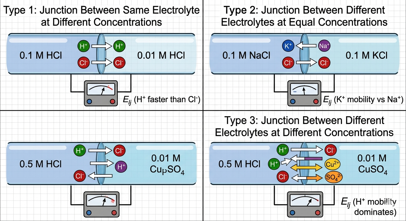
Figure 1: Visual comparison of the three primary modes of liquid-liquid junctions across electrolyte concentration boundaries.
Mathematical Derivation and Calculation
Quantifying the liquid junction potential requires evaluating the thermodynamic work associated with transferring ions across a non-equilibrium boundary. The total liquid junction potential (E_{lj}) can be derived by integrating the structural framework of the Nernst-Planck equation across the thickness of the boundary zone. For a simple single electrolyte system with varying concentrations, the relation simplifies significantly into the standard form: E_{lj} = (2t_minus – 1) * (RT/F) * ln(a₂/a₁), where t_minus represents the transport number of the anion.
Interactive Single-Electrolyte LJP Calculator
Estimate the liquid junction potential for a 1:1 electrolyte at 25°C (298.15 K) based on its activity ratio and transport number.
Practical Examples and Reference Values
To understand how these potentials affect real-world measurements, look at the experimental values generated at 25°C for various common liquid interfaces:
| Solution 1 (Left Half) | Solution 2 (Right Half) | Measured E_{lj} at 25°C (mV) |
|---|---|---|
| 0.1 M HCl | 0.1 M KCl | +26.8 |
| 0.1 M HCl | 0.01 M HCl | +38.2 |
| 0.1 M NaCl | 0.1 M KCl | -6.4 |
| 0.1 M KCl | 0.1 M LiCl | +8.8 |
| 4.0 M KCl (Bridge) | 0.1 M HCl | +4.7 |
Minimizing Liquid Junction Potential: The Salt Bridge
In analytical electrochemistry, we often need to isolate the measured cell electromotive force (EMF) from extraneous interfacial variations. The primary tool used to minimize liquid junction potentials is the salt bridge. A classic salt bridge is a low-resistance pathway connecting two half-cells without letting them mix completely. It usually consists of a glass U-shaped tube or a flexible sleeve junction packed with a dense gel matrix. This gel is typically prepared using an inert, highly concentrated filling electrolyte (such as 3.0 M to saturated KCl) and a stabilizing polymer gel base like agar-agar.
Potassium chloride (KCl) is chosen as the standard bridge electrolyte because its ions are nearly equimobile; at room temperature, the transport number of K⁺ is approximately 0.490, and for Cl⁻ it is 0.510. Because their velocities are nearly identical, the internal potential mismatch generated within the bridge itself approaches zero. Furthermore, by maintaining a high saturated concentration, the ionic flux out of the bridge dominates the interface, lowering the total net liquid junction potential to just a few millivolts.
Conclusion
The liquid junction potential is a fundamental electrochemical phenomenon that occurs whenever differing electrolytic solutions meet. Driven by disparities in ionic mobility, it forms an electrical double layer that can alter cell voltage measurements. Fortunately, by using equimobile salt bridges or applying mathematical corrections like the Henderson equation, electrochemists can minimize or correct for these errors, ensuring the high precision required for modern analytical research.
Download Complete Notes Below
Proudly Powered By


Leave a Comment